In the realm of subsurface data visualization, the 10th anniversary of GeoToolkit.JS marks a significant milestone. What began as a comprehensive set of high-performance tools and libraries has evolved into an indispensable resource for developers seeking to craft advanced, domain-specific software efficiently.
GeoToolkit™ encompasses diverse features, catering to the complex needs of developers working with 2D/3D seismic, well log, schematics, contour, maps, charts, and more. Its flexibility allows embedding within energy applications or building from the ground up, facilitating swift and precise development. Also, integrating GeoToolkit.JS data visualization libraries within the oil and gas industry is a game-changer for the end user—be it a geoscientist, an engineer, or a decision-maker. These individuals rely on accurate, comprehensive insights derived from complex subsurface data.
This anniversary is not just a celebration of a decade but a commemoration of more than 30 years of GeoToolkit’s presence in the industry, with versions spanning .NET, Java, JavaScript / TypeScript, and C++. Over this period, GeoToolkit has continuously evolved, refining its capabilities and pushing the boundaries of subsurface data visualization.
The journey of GeoToolkit has been paved with remarkable achievements. Its key benefits include support for various subsurface data formats like LAS, DLIS, WITSML, SEG-Y, SEG-D, and more in some versions of GeoToolkit. Moreover, it provides robust technical support, extensive online documentation, and a thriving Developer Community, fostering collaboration and knowledge exchange.
GeoToolkit’s high-performance tools and libraries stand out for their plug-and-play nature. With just a single line of code, developers can deploy these tools or use them as the foundation for crafting custom applications, significantly expediting time-to-market.
The extensive capabilities of GeoToolkit cover a broad spectrum of functionalities, from 3D seismic and reservoir data visualization using WebGL technology to 2D scatter plots for comparison, well log displays that can correlate thousands of wells, and the creation of PDF reports with multiple widgets for streamlined log header construction.
Furthermore, its extensive volume rendering capability facilitates high-quality visualizations of massive datasets, enabling seamless visualization of billions of cells. GeoToolkit also boasts robust support for diverse map layers, such as Google, ESRI, Bing Maps, ArcGIS GeoServices, OpenStreetMap, and more, making it an invaluable asset for comprehensive geospatial applications.
Here’s a glimpse of the evolution of GeoToolkit.JS showcasing its transformative capabilities:
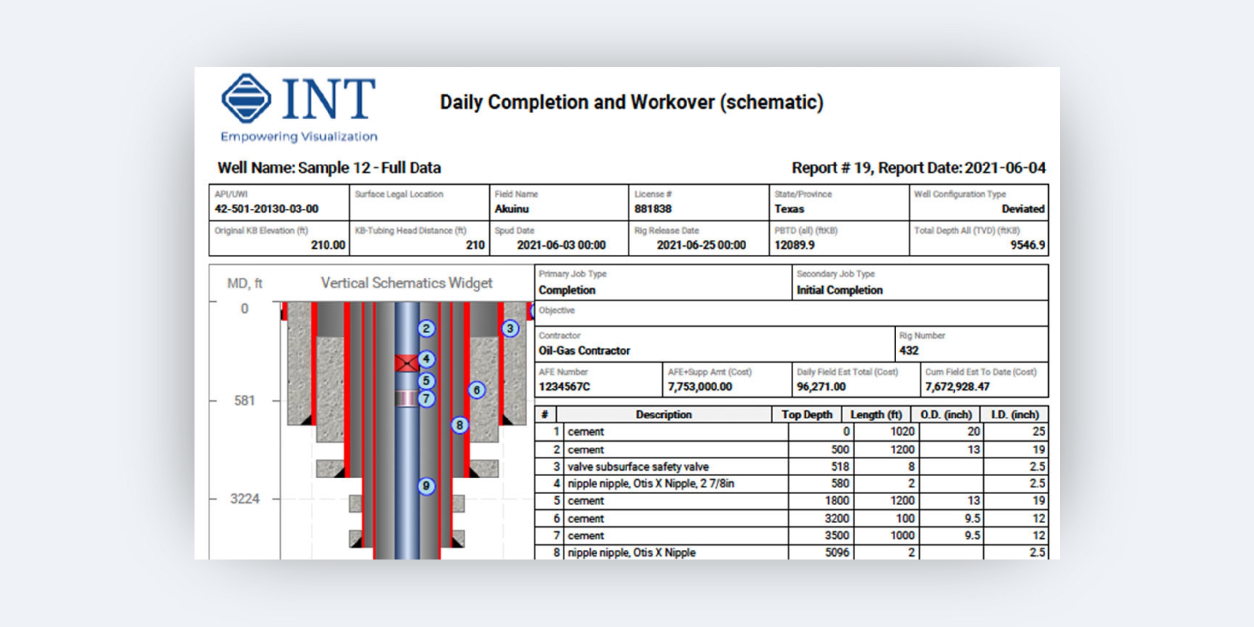
Report Builder
Build PDF reports with multiple widgets, including custom log headers, with template saving and printing for efficient creation and sharing.
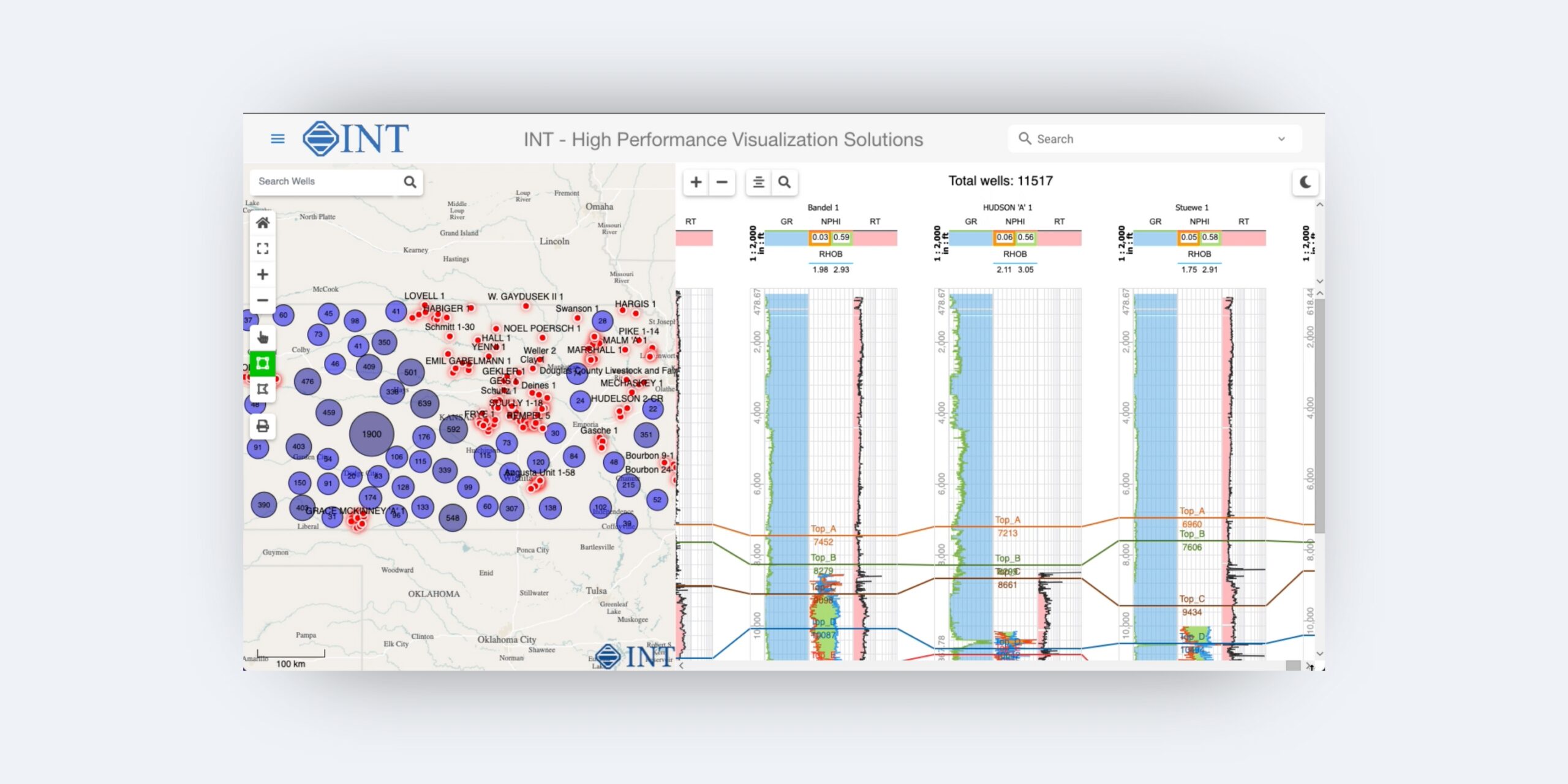
Well Log Correlation
Correlate thousands of wells effortlessly with well log displays, streamlining your analysis.
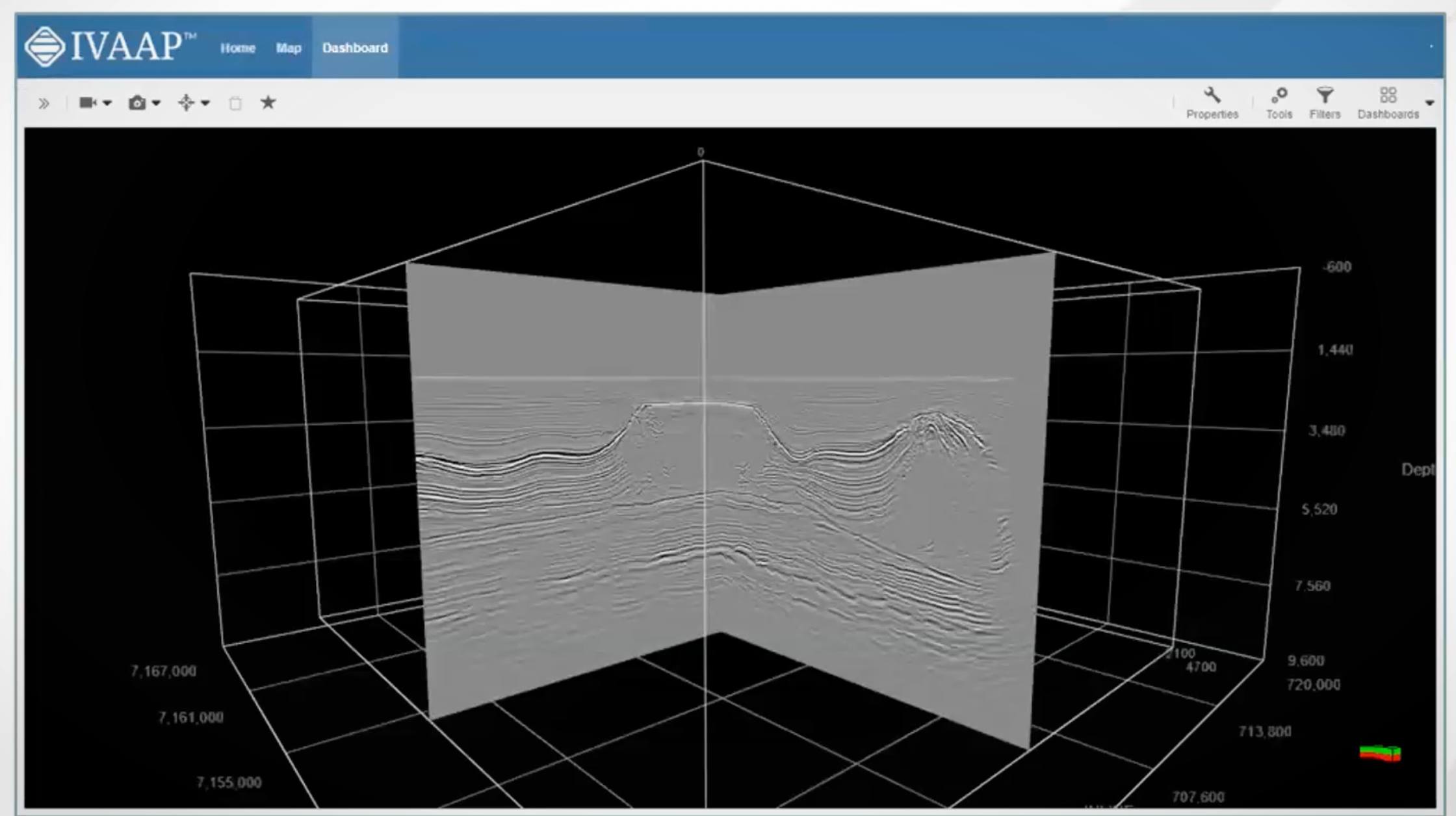
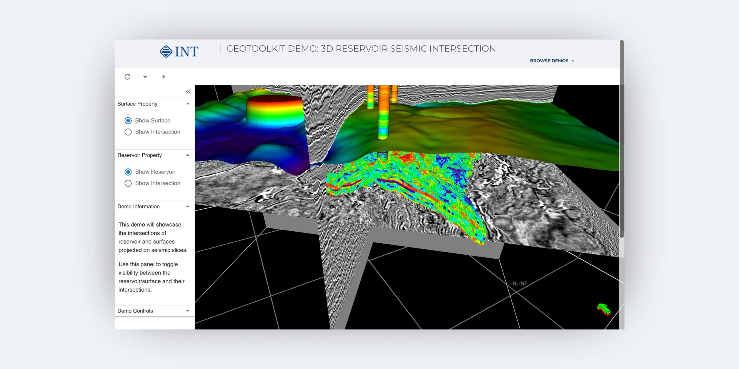
3D Reservoir Seismic Intersection
Intersect your 3D reservoir grid with seismic data and add well logs, horizons, and more.
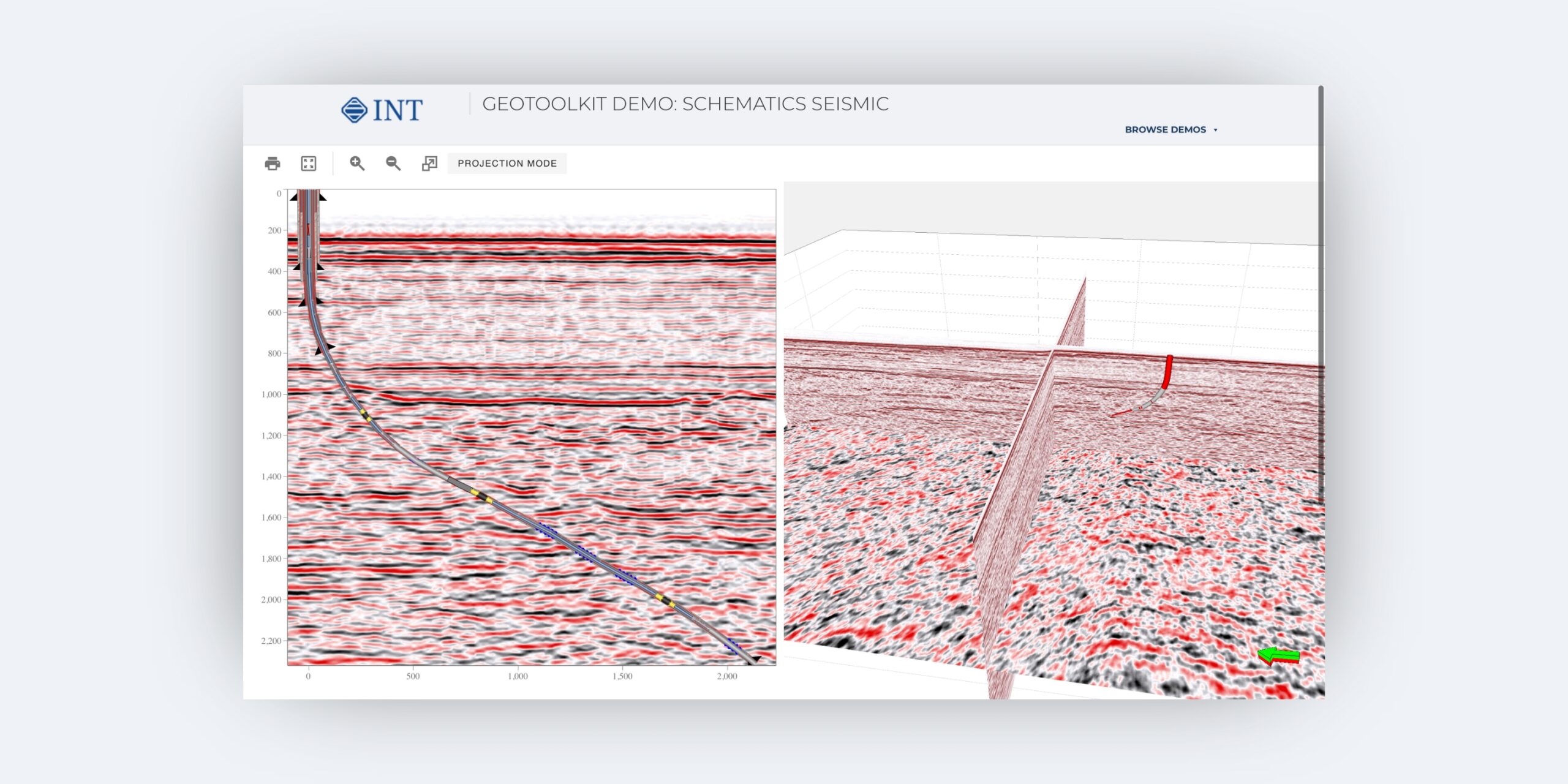
Schematics Seismic
Combining wellbore architecture with seismic profiles, this tool allows you to identify zones of interest in relation to each hole section and cementing sections versus formations crossed.
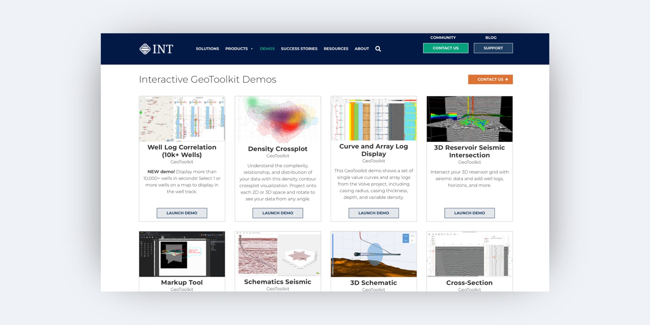
GeoToolkit Demo Gallery
Dive deeper and experience the transformative capabilities of GeoToolkit with our Interactive GeoToolkit Demos.
“Without INT’s GeoToolkit, we wouldn’t be where we are right now with C-Fields. We have high expectations that this tool will become the standard in Field Development planning and that we will be able to accomplish a lot with this tool. There’s nothing in the market like C-Fields right now.”
—Francisco Caycedo, Regional Director Latin America, CAYROS
However, amidst this celebration, expressing our deepest gratitude is crucial. To every individual involved in the development of GeoToolkit, your dedication, expertise, and unwavering commitment have been the cornerstone of our success. Your collective efforts have driven innovation, shaped the product, and paved the way for a decade of groundbreaking achievements.
To our clients, we extend our heartfelt thanks. Your trust, partnership, and continuous support have been the driving force behind GeoToolkit’s evolution.
The 10th anniversary of GeoToolkit.JS showcases innovation and an unwavering commitment to empowering developers in the intricate landscape of subsurface data visualization. Here’s to a decade of achievements and many more years of pioneering advancements in the field.
To learn more about GeoToolkit.JS, please visit int.com/products/geotoolkit/ or contact us at intinfo@int.com.
Explore our Interactive GeoToolkit Demos
Request a 30-day trial